Core Modeling at Instagram

At Instagram we have many Machine Learning teams. While they all work on different parts of the product, they all directly contribute to Instagram’s mission of strengthening relationships through shared experiences. This post is about one such team: Core Modeling.

Core Modeling’s mission is to increase the predictive power of models. This requires solid understanding of the fundamentals and models used, a mix of research and applied machine learning.

Here we summarize a few battle-tested methods we use to improve our models. Those are part of our core modeling arsenal and are commonly used here at Instagram.

Features

Features are representations of data in a machine learning model. Some of them are more important to the model, some less, and it’s often hard to know in advance which is which.

N-grams

N-grams are a contiguous sequence of n items from a given sample of text or speech.

Embeddings of n-grams using quantized dense features and categorical features that we jointly learn with the rest of our models have been very useful for us. There are two steps involved: creating the embeddings, and learning them with the model.

To create these embeddings, we first estimate the target cardinality for the n-grams, mostly dictated by model size capacity. We select the features by feature importance and smoothness of distribution, because rough distributions are harder to quantize. The embeddings are then randomly initiated for each bucket of the n-grams.

Finally, to jointly learn these embeddings, we have to make a model-dependent choice on how to combine these with the main prediction pipeline. For an MLP we could add the dot product of said embeddings with a hidden layer, then apply gradient descent. That would be a sparse neural network application.

All in all this is useful to learn higher order interactions between those important features and the rest. It forces the model to acknowledge those high order relationships and have the extra benefit of finding interesting representations that could be used in KNN/retrieval settings for those n-grams.

Embeddings

Learning low dimension representations of entities is not only useful for recommendations and retrieval, but also with helping models generalize better.

Because most prediction models are trained on a specific surface belonging to a larger product, training entity embeddings representing the holistic product experience brings a valuable source of meta information to myopic models. (In Instagram for example, the home feed or Explore would be one surface, where Instagram is the larger product.)

At Instagram we built different pipelines generating user embeddings that are used in both retrieval phases and point models. We mainly leverage two techniques to learn these embeddings:

• Word2Vec: We define the interactions that characterizes best our users, say a “like” is the interaction we are looking after. We then generate rows with list of users that have liked other users, for example if user1 liked user2 and user3 then we’d have a row with (user1, [user2, user3]). We define a notion of distance between users and train various versions of embeddings based on that idea.
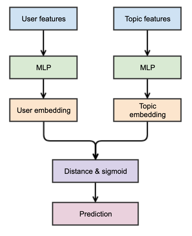
• Deep Learning: Neural networks naturally learn representations of features in hidden layers we leverage a multi tower like architecture as shown below. This allows us to scale our embeddings to very high coverage since it’s not only fast to compute but we can also load those embeddings offline allowing for lightning fast (using FAISS) similarity search at inference time.

Pooling and hashing

One difficulty of integrating those embeddings in a model is that we usually have a mixture of embeddings that we need to merge — or “pool” — together into one.

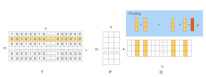
For example: if we are building a neural network to predict the probability of a viewer commenting on a media as part of its sparse features the network will be fed a list of the last N user IDs on whose content this viewer commented. The neural network will then have to learn a representation for each user.

This could be done using the method illustrated below where the network performs a decomposition of a sparse matrix to get embeddings for users with whom this user has interacted, then a pooling layer would blend these together to represent the centroid of the users on whose content this user has commented.

The assumption is that the closer (as in distance) a new user is to that centroid, the more likely that new user would be to comment upon their content.

There are a few important hyper-parameters to this method.

• Hashing: First the model needs to hash the user IDs into a predefined, countable set. This can be tricky as some user IDs occurs more often than others, e.g. if those users post more or have more followers. Therefore, to have even coverage, it’s important that they don’t end up in the same hashed bucket. This led us to work on a better hashing strategy which took frequency into account.
• Dimensionality: We also have to factor in the embeddings dimension. Given that there are many users and that the model needs to have a lookup table of the embeddings in memory this gives strong restrictions on the embeddings size as we have |hash_users_size| x |embeddings_dimension| floats to store. To keep models lean and efficient we have tools that monitor the cardinality of each of our sparse features. Those tools can automatically perform dimensionality reductions on the learned embeddings , and alert if we are off in terms of dimensionality or hash size.
• Pooling: There are many well-known pooling methods (attention, sum, average, max, etc.) to aggregate those hidden states. They are all semantically different. This is still somewhat a “black box” for us, an area for understanding and development. For now, we usually tune this with our general bayesian optimization of hyper-parameters.

Fundamentals

We see some similar patterns over and over again across our machine learning teams. The below fundamentals come up often enough that want to share our approach in the hopes it helps others.

Cold start and bootstrapping

But first, what is the “cold start” problem?

Example: Let’s imagine you use one of the methods mentioned earlier and you have generated embeddings. Now you want to predict whether a user will be interested in buying a product. To do that you compute the dot product between the two embeddings and use that as your prediction

This can work well in practice, but what happens when a new user or product appears and you don’t have embeddings generated for them yet? Or simply don’t have enough data to even generate the embeddings? This is the cold start problem.

If the models used for a task are using historical features, or features who do not have coverage for new use-cases, their predictive power will be subpar. There are a few ways to deal with such cases.
At Instagram we monitor feature coverage fed into a model and if it is lower than a threshold we have fallback options that are less accurate but only use high fidelity features. We are also in the process of building mixture embeddings on user clusters, those have full coverage and are a good substitute for interaction history. Coming up we will be baking this into our training pipelines where each feature will have a “reliability” score and we will automatically produce fallback models for every model trained.

Offline vs Online vs Recurring

In many cases the products and the ecosystem are highly non-stationary, seasonal, and sensitive to trends. Therefore training a model offline leads to a “stale” prediction whose accuracy likely deteriorates over time. At Instagram we usually have two types of model updates:

• Recurring: Periodically (typically daily) a model will load the past N days of training data (N is usually 1 or 7), and keep training by loading the previous “snapshot” of the previous period. The model would keep propagating the gradients as if it was simply training on more data. The snapshot is then published and our inference infrastructure immediately picks it up for production purposes.
• Online: Here the model will actually be fed realtime data and will update itself often. We usually use online training for domains that are highly sensitive to trends. We get guaranteed freshness at a high engineering and maintenance cost. The pipeline to compute and update real time data may be resource-intensive.

Recurring training provides a few advantages. It’s fairly painless to have an up-to-date model since it leverages the existing training methods. It’s also less resource-intensive since all the data is computed offline, doesn’t have to be there in real time. There may also be a computational cost to setting up proper vetting criteria to publish a snapshot. We usually evaluate against a fixed golden set, and a changing test set, as a good practice.

Both of these methods have caveats, too. Depending on which gradient descent method and learning rate you use, your model may not be really updating after a significant number of days. For example by using Adagrad the square of the gradients will keep increasing until updates become non-meaningful. On the other hand you also usually want some resilience to new data. In particular a new bad day of data shouldn’t throw off the models too much.
At Instagram we built a tool to monitor the correlations between weights and predictions between each snapshots on a fixed training data set and a held out in time one, this allows us to control for the learning rate and optimization methods mentioned above as well as detecting bad snapshots before they get published. It also helps us notice if our underlying training data has suddenly changed and model performance is affected. We can then use our other tools to inspect the data and pin point what specifically changed.

Mixture of experts and sub-models

It is common at the scale of Instagram to see sub-populations of users behaving very differently for a given prediction tasks. For instance, users in country A may have a higher like rate than in country B. Machine learning usually handle these things pretty well by learning those disparities, however sometimes it is highly useful to handle those cases separately.

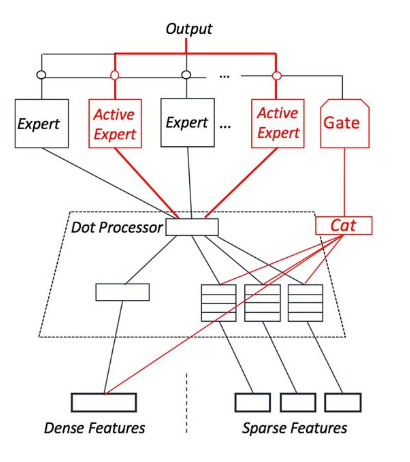
One idea to tackle this is by aggregating distributions and statistics for features and labels, then computing a Kullback–Leibler divergence between sub-populations to monitor how divergent they are. If we decide that a sub-population is behaving differently enough that it warrants special attention, we usually resort to a sparsely gated mixture of expert type of models where a gate can learn which experts to activate at inference time as a function of the input features.

Offline analysis and backtesting

As soon as a machine learning pipeline becomes mature the iteration speed matters even more. It takes more and more effort for increasingly marginal gains. Therefore, assessing quickly how a model or value model is performing is key to the teams’ success.

More than that it is critical to understand the ecosystem consequences of an experiment in depth to properly reason about causality, thereby avoiding engineers blindly performing a random walk along the path of hyper-parameters.

We have built a cohesive tool that replays past traffic using control and test treatments, and computes a panel of ecosystem and model metrics to help engineers with their project. This allows an engineer to quickly check that the expected results are moving in the intended fashion.

We are now working on predicting how an online experiment is doing by leveraging those offline metrics to reduce iteration speed even more. More on that in a future post.

Ranking-specific practices

Ranking use cases arises naturally on our platform and therefore we wanted to share some ranking-specific practices that have proven useful for us.

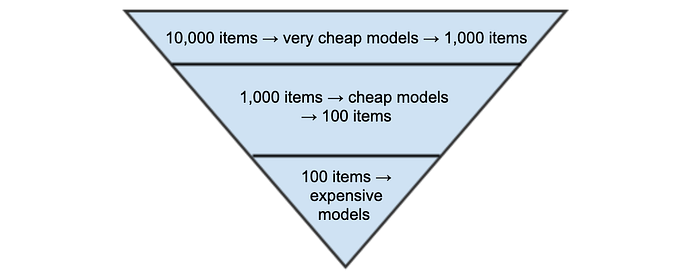
• Multi-stage ranking: At our scale model size and inference speed is important and resource-intensive. The inventory we rank is large, so it is computationally impossible to perform complex inference on a large set of items. For these reasons we usually set up multi-stage ranking as soon as the inventory or request volume go past a certain threshold.
• The idea is to use a simpler model as first pass on many items, then pick the top N items (N much smaller than the original amount of items) on which we perform the more resource-intensive inference. Our preferred 0-pass or 1-pass models are either dot products between embeddings (simple and fast) or small LambdaRank models

• Loss function and inverse propensity weighting: When the ranked list of items doesn’t have a human-generatable ideal relevant ranking (unlike most information theory cases), most pipelines default to point-wise models instead of Learning-To-Rank framework.
• For instance, one might rank the Instagram stories by computing P[tapping on the story] for each available medias and sorting by the probability. This works pretty well, albeit the loss function becomes an issue, because in most ranking use-cases the top items are much more impactful than the rest.
• At training time the loss function will optimize for examples, regardless of their position. Then one might find a situation where of the two models, one has a better validation performance than the other, yet performs worse online. That happens because the model is doing slightly worse for the high scores and much better for the lower scores. We have a couple methods to deal with this. The simplest approach is to borrow ideas from inverse propensity weighting and weight training examples by their positions. This helps skew the loss function towards meaningful errors.
• Bias features: Data bias is usually high for ranking use-cases. The action you are trying to model is predominant for items at the top of the list. For example, the like rate for the first post is higher than for post #20. To deal with this we often add position and batch size in the last layer of a neural network, or to co-train your model with a logistic regression using these features, to help the model account for this bias.
• The latter formulation allows us to do position ranking on a large set of items. One can perform model inference once for all items then pick the best one at position 0. Then simply perform inference again on the small logistic regression to find the best pick for position 1, and so on.

Parting words

We hope that you found this informative and helpful. These projects are a sample of the work done by our modeling teams, who are consistently inspired by research, and take advantage of the wealth of data we have at Instagram. There are a few on-going projects that we will detail in future blog posts, so please share comments, feedback, and requests.