Trending on Instagram

With last week’s Search and Explore launch, we introduced the ability to easily find interesting moments on Instagram as they happen in the world. The trending hashtags and places you see in Explore surface some of the best, most popular content from across the community, and pull from places and accounts you might not have seen otherwise. Building a system that can parse over 70m new photos each day from over 200m people was a challenge. Here’s a look at how we approached identifying, ranking, and presenting the best trending content on Instagram.

Definition of a trend

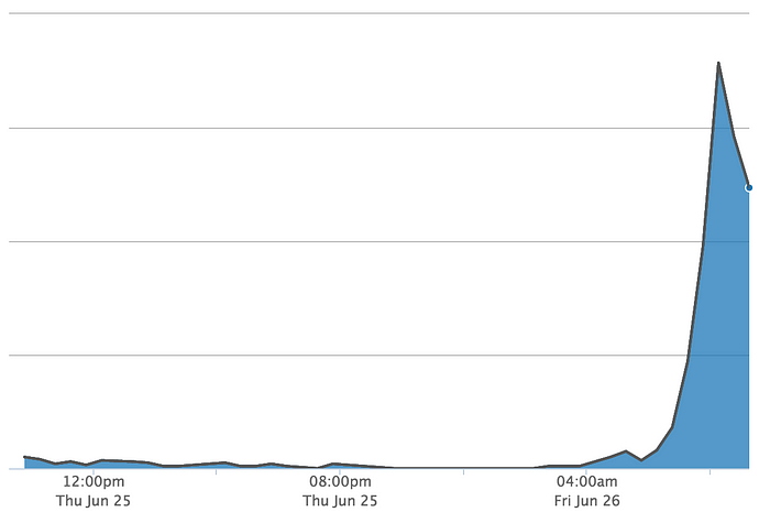
Intuitively, a trending hashtag should be one that is being used more than usual, as a result of something specific that is happening in that moment. For example, people don’t usually post about the Aurora Borealis, but on the day we launched, a significant group of people was sharing amazing photos using the hashtag #northernlights. You can see how usage of that hashtag increases over time in the graph below.

And as we write this blog post, #equality is the top trending hashtag on Instagram.

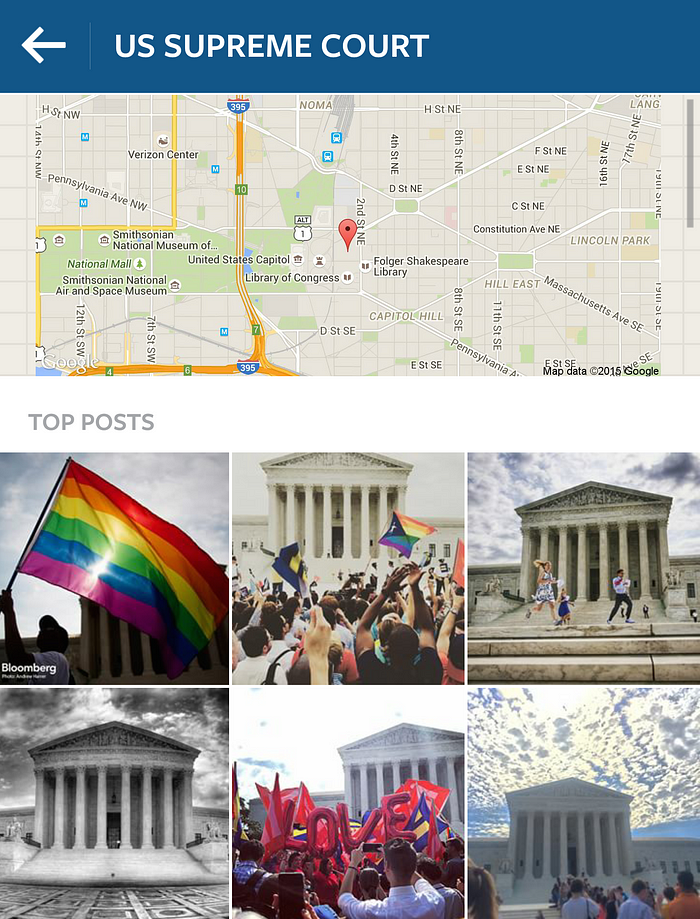
Similarly, a place is trending whenever there is an unusual number of people who share photos or videos taken at that place in a given moment. The U.S. Supreme Court is trending, as there are hundreds of people physically there sharing their support on the recent decision in favor of same-sex marriage.

Given examples such as the above, we identified three main elements to a good trend:

• Popularity — the trend should be of interest to many people in our community.
• Novelty — the trend should be about something new. People were not posting about it before, or at least not with the same intensity.
• Timeliness — the trend should surface on Instagram while the real event is taking place.

Overall, we want major events like #nbafinals or #nyfashionweek to trend, together with the places they happen, as soon as they start and as long as the community is interested in them.

In this post we discuss the algorithms we use and the system we built to identify trends, rank them and show them in the app.

Identifying a trend

Identifying a trend requires us to quantify how different the currently observed activity (number of shared photos and videos) is compared to an estimate of what the expected activity is. Generally speaking, if the observed activity is considerably higher than the expected activity, then we can determine that this is something that is trending, and we can rank trends by their difference from the expected values.

Let’s go back to our #northernlights example in the beginning of this post. Regularly, we observe only a few photos and videos using that hashtag on an hourly basis. For #northernlights, starting at 07:00am (Pacific time), thousands of people shared content using that hashtag. That means that activity in #northernlights is well above what we expect. Conversely, more than 100k photos and videos are tagged with #love every day, as it is a very popular hashtag. Even if we observe 10k extra posts today, it won’t be enough to exceed our expectations given its historical counts.

For each hashtag and place, we store counters of how many pieces of media were shared using the hashtag or place in a 5-minute window over the past 7 days. For simplicity, let us focus on hashtags for now, and let’s assume that C(h, t) is the counter for hashtag h at timet (i.e., it is the number of posts that were tagged with this hashtag since time t-5min till timet). Since this count varies a lot between different hashtags and over time, we normalize it and compute the probability P(h, t) of observing the hashtag h at time t.

Given the historical counters of a hashtag (aka the time series), we can build a model that predicts the expected number of observations: C’(h, t), and similarly, compute the expected probability P’(h, t). Given these two values for each hashtag, a common measure for the difference between probabilities is the KL divergence, which in our case is computed as:

S(h, t) = P(h, t) * ln(P(h, t)/P’(h, t))

What this does is essentially consider both the currently observed popularity, which is captured by P(h, t), and the novelty, computed as the ratio between our current observations and the expected baseline, P(h, t)/P’(h, t). The natural log (ln) function is used to smooth the “strength” of novelty and make it comparable to the popularity. The timeliness role is played by the t parameter, and by looking at the counters in the most recent time windows, trends will be picked up in real-time.

A prediction problem

How do you compute the expected baseline probability given past observations?

There are several facets that can influence the accuracy of the estimate and the time-and-space complexity of the computation. Usually those things don’t get along too well — the more accurate you want to be, the more time-and-space complexity the algorithm requires. So we had to be careful when considering the number of samples (how far back we look), the granularity of sample (do we really need counts every five minutes?) and how fancy the algorithm should be. We experimented with a few different alternatives, like simply taking the count of the same hour last week, and also regression models up to crazy all-knowing neural networks. Turns out that while fancy things tend to have better accuracy, simple things work out well, so we ended up with selecting the maximal probability over the past week’s worth of measurements. Why is this good?

• Very easy to compute and relatively low memory demand.
• Quite aggressive about suppressing non-trends with high variance.
• Quickly identifies emerging trends.

There are two things we over-simplified in this explanation, so let us refine our model a bit more.

First, while some hashtags are extremely popular and have lots of media, most of the hashtags are not popular, and the 5-minute counters are extremely low or zero. Thus, we keep an hourly granularity for older counts, as we don’t need a 5-minute resolution when computing the baseline probability. We also look at a few hours worth of data so that we can minimize the “noise” caused by random usage spikes. We noted there is a trade-off between the need to get sufficient data and how quickly we can detect trends — the longer the time frame is, the more data we have, but the slower it will be to identify a trend.

Second, if the predicted baseline P(h, t) is still zero, even after accumulating a few hours for each hashtag, we will not be able to compute the KL divergence measure (division by zero). Hence we apply smoothing, or put more simply: If we didn’t see any media for a given hashtag in the past, we mark it as if we saw three posts in that timeframe. Why *three* exactly? That allows us to save a large amount of memory (>90%) while storing the counters, as the majority of hashtags do not get more than three posts per hour, so we can simply drop the counters for all of those and assume every hashtag starts with at least three posts per hour.

Even with all that memory savings, there is a lot of data to store. Instagram sees millions of hashtags per day, and several tens of thousands of places. We want the trending backend to respond quickly and scale well with our growth, so we designed a sharded stream processing architecture that we explain later.

Ranking and Blending

The next step is to rank the hashtags based on their “trendiness,” which we do by aggregating all the candidate hashtags for a given country/language (the product is enabled in the USA for now) and sorting them according to their KL divergence score, *S(h, t)*. We then impose a lower-bound so that we drop all candidates below a certain score. This way we get rid of non-interesting trends and create a smaller list of interesting trends.

We noticed that some trends tend to disappear faster than the interest around them. For instance, the amount of posts using a hashtag that is trending at the moment will naturally decrease as soon as the event is finished. Therefore, its KL score will quickly decrease, then the hashtag won’t be trending anymore, even though people usually like to see photos and videos from the underlying event of a trend for a few hours after it is over.

In order to overcome those issues, we use an exponential decay function to define the time-to-live for previous trends, or how long we want to keep them for. We keep track of the maximal KL score for each trend, say SM(h), and the time tmax where S(h, tmax) = SM(h). Then, we also compute the exponential decayed value for SM(h) for each candidate hashtag at the moment so that we can blend it with their most recent KL scores.

Sd(h, t) = SM(h) * (1/2)^((t — tmax)/half-life)

We set the decay parameter *half-life* to be two hours, meaning that SM(h) is halved every two hours. This way, if a hashtag or a place was a big trend a few hours ago, it may still show up as trending alongside the most recent trends.

Grouping similar trends

People tend to use a range of different hashtags to describe the same event, and when the event is popular, multiple hashtags that describe the same event might all be trending. Since showing multiple hashtags that describe the same event can end up being an annoying user experience, we group together hashtags that are “conceptually” the same.

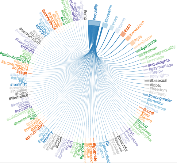
For example, the figure illustrates all the hashtags that were used in media together with #equality. It shows that #equality was trending together with related hashtags, such as #lovewins, #love, #pride, #lgbt and many others. By grouping these tags together, we can show #equality as the trend, and save the need to sift through all the different tags until reaching other interesting trends.

To do this, there are two important tasks that need to be achieved — first, understand which hashtags are talking about the same thing, and second, find the hashtag that is the best representative of the group. In slightly more “scientific” terms, we need to capture the affinities between hashtags, cluster them based on these affinities, and find an exemplar point that describes each cluster. There are two key challenges here — first we need to capture some notion of similarity between hashtags, and then we need to cluster them in an “unsupervised” way, meaning that we have no idea how many clusters there should be at any given time.

We use the following notion of similarity between hashtags:

• Cooccurrences — hashtags that tend to be used together (cooccur on the same piece of media) — for example #fashionweek, #dress, #model. Cooccurrences are computed by looking at recent media and counting the number of times each hashtag appears together with other hashtags.
• Edit distance — different spellings (or typos) of the same hashtag — for example #valentineday, #valentinesday — these tend not to cooccur because people rarely use both together. Spelling variations are taken care of using Levenshtein distance.
• Topic distribution — hashtags that describe the same event — for example #gocavs, #gowarriors — these have different spelling and they are not likely to cooccur. We look at the captions used with these hashtags and run an internal tool that classifies them into a predefined set of topics. For each hashtag we look at the topic distribution (collected from all the media captions in which it appeared) and normalize it using TF-IDF.

Our hashtag grouping process computes the different similarity metrics for each pair of trending hashtags, and then decides which two are similar enough to be considered the same. During the merging process, clusters of tags emerge, and often these clusters will also be merged if they are sufficiently similar.

Now that we have talked about the entire process for identifying trends at Instagram, let us take a look at how the backend was implemented in order to incorporate each component described above.

System design

Our trending backend is designed as a stream processing application with four nodes, which are connected in a linear structure like an assembly line, see the top part of this diagram:

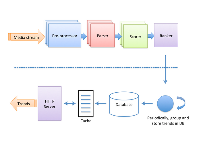
Nodes consumes and produces a stream of “log” lines. The entry point receives a stream of media creation events, and the last node outputs a ranked list of trending items (hashtags or places). Each node has a specific role as follows:

• pre-processor — the original media creation events holds metadata about the content and its creator, and in the pre-processing phase we fetch and attach to it all the data that is needed in order to apply quality filters in the next step.
• parser — extracts the hashtags used in a photo or video so that each one of them becomes a separate line in the output stream. This is where most of the quality filters are applied, so if a post violates any of them, it is simply ignored.
• scorer — stores time-aggregated counters for each hashtag. The counters are all kept in memory, and they are also persisted into a database so that they can be recovered in case the process dies. This is also where our scoring function S(h, t) is computed. Every five minutes, a line is emitted that contains each hashtag and its current value for S(h, t).
• ranker — aggregates all the candidate hashtags and their trending scores. Each hashtag has actually two possible scores: their current values and their exponential decayed values based on their historical maximum, Sd(h, t) as described above.

This stream-lined architecture lets us partition the universe of hashtags so that there can be many instances of each node running in parallel, each one of them taking care of a different partition. That is desirable as the scorer is memory-bound and the amount of data may be too big to fit into a single machine. Besides, failures are isolated to specific partitions, so if one instance is not available at the moment, trending would not be entirely compromised.

Besides, We need to make sure the scorer’s input is partitioned properly so that all streamed log lines for a given hashtag are processed by the same exact instance, otherwise the counters for one hashtag would be split among several instances.

We wanted to serve requests for trending hashtags and places without imposing a considerably high load on our trending backend. Therefore, trends are served out of a read-through caching layer powered by memcached, and a Postgres database in case there is a cache miss, see the bottom part of the diagram above. Trends are periodically pulled from the ranker, then we run our algorithm to group similar trends together and the results are stored in Postgres, that’s how new trending hashtags and places are flushed into the app.